This page was generated from the Jupyter notebook gate_family_quick_start.ipynb. Open in Google Colab.

Gate Family Quick Start

Let us create one pulse family that implements controlled-phase gates,

\[\mathrm{CP}(\theta)=\operatorname{diag}(1,1,1,e^{i\theta}),\]

for several target phases \(\theta\). We use PulseFamilyAnsatz so the pulse duration and ansatz parameters are smooth functions of the CP phase.

# %pip install -q --progress-bar off rydopt # Uncomment for installation on Colab

import numpy as np
import rydopt as ro
import jax
import matplotlib.pyplot as plt

First, we choose target phases between \(0.05\pi\) and \(\pi\) that should be realized by the same family of pulses. Each phase defines one TwoQubitGate. We leave the single-qubit phase phi unspecified, so RydOpt may absorb any accompanying local \(Z\) phase. The GateFamily combines their infidelities during optimization using a softmax reduction, which is controlled by the reduction parameter that sets the scale of per-gate infidelity differences that the optimizer should care about. We choose a value that is one order of magnitude smaller than the target infidelity that we will set later for the optimization.

target_phases = np.linspace(0.05, 1, 9) * np.pi

sampled_gates = [
    ro.gates.TwoQubitGate(
        phi=None,
        theta=phase,
        Vnn=float("inf"),
        decay=0.0,
    )
    for phase in target_phases
]

gate_family = ro.gates.GateFamily(
    fixed_argument_gates=sampled_gates,
    argument_values=target_phases,
    reduction="softmax",
    softmax_scale=1e-4,
)

Then we choose a pulse family ansatz. The underlying pulse has constant detuning and a sine-CRAB laser-phase sweep with two coefficients. By default, the PolynomialPulseMapWithCustomDuration uses an empirical expression with three parameters for interpolating the duration as a function of the target phase. The detuning, laser-phase coefficients, and Rabi frequency amplitude are polynomial functions of the target phase. The degrees 0, 2, 0 of the polynomials keep the detuning phase-independent and make each laser-phase coefficient quadratic. The Rabi frequency amplitude remains fixed at one.

degrees = [3, 0, 2, 0]  # duration, detuning, laser phase, Rabi amplitude

pulse_map = ro.pulses.PolynomialPulseMapWithCustomDuration(degrees=degrees)
pulse_family = ro.pulses.PulseFamilyAnsatz(
    detuning_ansatz=ro.pulses.Const(),
    phase_ansatz=ro.pulses.SinCrab(2),
    pulse_map=pulse_map,
)

For multi-start optimization, we provide lower and upper bounds for random pulse-family parameters rather than a single initial guess. The bounds follow the map shapes: three duration parameters, one constant detuning coefficient, two quadratic laser-phase coefficients, and no trainable Rabi parameters.

min_initial_params = ro.pulses.PulseFamilyParams(
    [7, 16, 0.2], [[-0.1]], [[-5.0, -5.0, -5.0], [-5.0, -5.0, -5.0]], [[]]
)
max_initial_params = ro.pulses.PulseFamilyParams(
    [8, 17, 0.3], [[0.0]], [[5.0, 5.0, 5.0], [5.0, 5.0, 5.0]], [[]]
)

Now, we optimize the pulse-family parameters with multi_start_optimize. The optimizer samples random initial parameter sets within the bounds, runs each candidate for up to 1000 steps, and minimizes the mean infidelity over the training CP gates. Because the widths of the initialization bounds span two orders of magnitude (from 0.1 to 10), we set rescale=True, which scales each parameter’s update step by the width of its initialization interval. Then all parameters move a comparable fraction of their plausible range per step, improving convergence. To keep the runtime reasonable for this quick-start example, we set a target fidelity of \(10^{-3}\). Higher fidelities can be achieved by using a pulse family ansatz with more parameters and increasing the number of optimization steps and initializations.

opt_result_gate_family = ro.optimization.multi_start_optimize(
    gate_family,
    pulse_family,
    min_initial_params,
    max_initial_params,
    rescale=True,
    tol=1e-3,
    num_initializations=80,
    num_steps=1000,
    num_processes=4,
    return_history=False,
    learning_rate=0.02,
)
optimized_family_params = opt_result_gate_family.params

Started optimization using 4 processes

=== Optimization finished using multi-start Adam ===

Runtime: 320.347 seconds
Gates with infidelity below tol=1.0e-03: 9

Slowest gate:
> infidelity <= tol
PulseFamilyParams(
  duration_params = [16.79492764, 19.544852  , -0.03658006],
  detuning_params = [-0.36887261],
  phase_params =    [[-0.7136082 ,  0.54734925,  1.66779244],
                     [-3.74666949,  3.460282  ,  2.91358954]],
  rabi_params =     []
)

Fastest gate:
> infidelity <= tol
PulseFamilyParams(
  duration_params = [ 7.64772846, 15.56779742,  0.29144484],
  detuning_params = [-0.05752019],
  phase_params =    [[ 0.05856142, -1.60975399,  4.25004505],
                     [-2.47653115,  4.08420197, -1.47451204]],
  rabi_params =     []
)
> one-sided bootstrap error on duration: 0.009

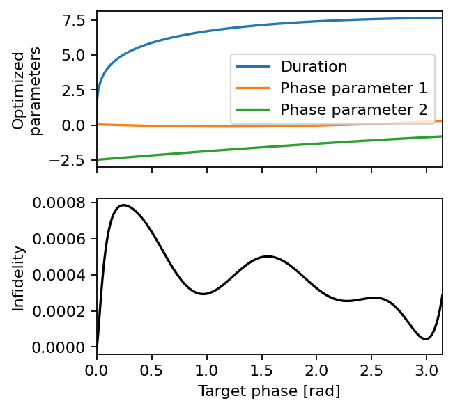
Finally, we inspect generated pulses on a fine phase grid. generate_pulse_params evaluates the polynomial map to obtain the single-pulse parameters corresponding to a target phase. Evaluating phases beyond the training points checks how well the optimized family interpolates.

phases = np.linspace(0, 1, 1000) * np.pi
durations = []
parameters = []
infidelities = []


@jax.jit
def analyze_phase(
    phase: float, family_params: ro.pulses.PulseFamilyParams
) -> tuple[jax.Array, jax.Array, jax.Array]:
    pulse = pulse_family.pulse_ansatz
    params = pulse_family.generate_pulse_params(family_params, phase)
    gate = ro.gates.TwoQubitGate(
        phi=None,
        theta=phase,
        Vnn=float("inf"),
        decay=0,
    )
    infidelity = 1 - ro.simulation.process_fidelity(gate, pulse, params)
    return params.duration[0], params.phase_params, infidelity


for phase in phases:
    duration, phase_params, infidelity = analyze_phase(phase, optimized_family_params)
    durations.append(float(duration))
    parameters.append(np.asarray(phase_params))
    infidelities.append(float(infidelity))

fig, (ax1, ax2) = plt.subplots(2, 1, sharex=True, figsize=(4, 4), dpi=160)
ax1.plot(phases, durations, label="Duration")
ax1.plot(
    phases,
    parameters,
    label=[f"Phase parameter {i + 1}" for i in range(len(parameters[0]))],
)
ax1.set_ylabel("Optimized\nparameters")
ax1.legend(loc="center right", fontsize=7)
ax2.plot(phases, infidelities, "k-")
ax2.set_xlim(phases[0], phases[-1])
ax2.set_ylabel("Infidelity")
ax2.set_xlabel("Target phase [rad]");

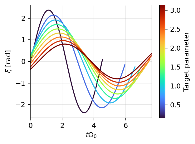
We can also plot the optimized phase sweeps for the target phases in gate_family. The detuning and Rabi functions are hidden because they are fixed or phase-independent in this ansatz.

ro.characterization.plot_pulse_family(
    pulse_family,
    optimized_family_params,
    gate_family,
    plot_detuning=False,
    plot_rabi=False,
);