This page was generated from the Jupyter notebook smooth.ipynb. Open in Google Colab.

Smooth Pulse

Let us implement a CZ gate on two atoms in the perfect Rydberg blockade regime, using smooth pulse ansatz functions for the phase and amplitude.

# %pip install -q --progress-bar off rydopt # Uncomment for installation on Colab

import rydopt as ro
import numpy as np
import matplotlib.pyplot as plt

First, we create the target gate.

gate = ro.gates.TwoQubitGate(phi=None, theta=np.pi, Vnn=float("inf"), decay=0.0)

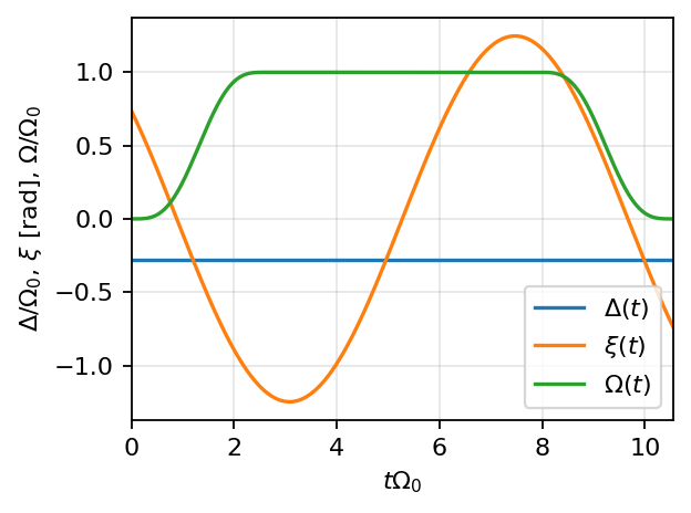
Then we choose a pulse ansatz that consists of a constant detuning, a sweep of the laser phase, and a smooth switching of the Rabi frequency amplitude. We provide initial guesses of pulse parameters as input for the optimization. For the Rabi frequency amplitude, we fix the pulse parameters so that the pulse plateaus at \(1\;\Omega_0\) and 50 % of the pulse duration is used for switching.

pulse_ansatz = ro.pulses.PulseAnsatz(
    detuning_ansatz=ro.pulses.Const(),
    phase_ansatz=ro.pulses.SinCrab(2),
    rabi_ansatz=ro.pulses.SoftBoxSeventhOrderSmoothstep(),
)

initial_params = ro.pulses.PulseParams(12.0, [0.0], [0.0, 0.0], [1.0, 0.5])
fixed_initial_params = ro.pulses.PulseParams(
    False,
    [False],
    [False, False],
    [True, True],
)

Now, we perform the optimization and plot the result.

opt_result = ro.optimization.optimize(
    gate, pulse_ansatz, initial_params, fixed_initial_params
)
optimized_params = opt_result.params

ro.characterization.plot_pulse(pulse_ansatz, optimized_params);

Started optimization using 1 process

=== Optimization finished using Adam ===

Duration: 6.599 seconds
Gates with infidelity below tol=1.0e-07: 1

Optimized gate:
> infidelity <= tol
> parameters = (10.55125730334775, [0.28121562], [0.42764051 1.24775025], [1.  0.5])
> duration = 10.55125730334775

We can also show the spectrum of the pulse.

ro.characterization.plot_spectrum(pulse_ansatz, optimized_params);

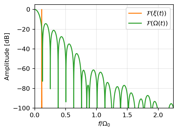
In the code, we used a soft-box pulse ansatz with 7th-order-smoothstep-shaped edges. For several examples of soft-box pulse ansatze and their spectra, see below.

ansatze = [
    ro.pulses.PulseAnsatz(rabi_ansatz=ro.pulses.SoftBoxHann()),
    ro.pulses.PulseAnsatz(rabi_ansatz=ro.pulses.SoftBoxPlanck()),
    ro.pulses.PulseAnsatz(rabi_ansatz=ro.pulses.SoftBoxSeventhOrderSmoothstep()),
]
labels = [
    "softbox_hann",
    "softbox_planck",
    "softbox_seventh_order_smoothstep",
]

fig, ax = plt.subplots(figsize=(4, 3), dpi=160)

for ansatz in ansatze:
    params = ro.pulses.PulseParams(15.0, [], [], [1.0, 0.5])
    ro.characterization.plot_spectrum(ansatz, params, ax=ax)

for line, label in zip(ax.get_lines(), labels):
    line.set_label(label)

ax.legend(fontsize=8)
ax.set_xlim(0, 4)
ax.set_ylim(-100, 5)
ax.set_xlabel(r"$f / \Omega_0$")
ax.set_ylabel("Amplitude (dB)")
ax.grid(alpha=0.3)